In the Introduction: Simulink Modeling page we demonstrated how Simulink can be employed to simulate a physical system. More generally, Simulink can also simulate the complete control system, including the control algorithm in addition to the physical plant. As mentioned previously, Simulink is especially useful for generating the approximate solutions of mathematical models that may be prohibitively difficult to solve "by hand." For example, consider that you have a nonlinear plant. A common approach is to generate a linear approximation of the plant and then use the linearized model to design a controller using analytical techniques. Simulink can then be employed to simulate the performance of your controller when applied to the full nonlinear model. Simulink can be employed for generating the linearized model and MATLAB can be employed for designing the controller as described in the other Introduction pages. Various control design facilities of MATLAB can also be accessed directly from within Simulink. We will demonstrate both approaches in this page.
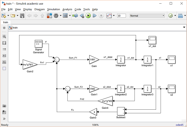
Recall the Simulink model of the toy train system derived in the Introduction: Simulink Modeling page and pictured below.

You can generate this model yourself, or you can download the completed model by right-clicking here and then selecting Save link as .... Assuming that the train only travels in one dimension (along the track), we want to apply control to the train engine so that it starts and comes to rest smoothly, and so that it can track a constant speed command with minimal error in steady state.
Let us first create the structure for simulating the train system in unity feedback with a PID controller. In order to make our Simulink model more understandable, we will first save the train model into its own subsystem block. To accomplish this, delete the three scope blocks and replace each one by an Out1 block from the Sinks library. Label each Out1 block with the corresponding variable name, "x1_dot", "x1", and "x2". Then delete the Signal Generator block and replace it with an In1 block from the Sources library. Label this input "F" for the force generated between the train engine and the railroad track. Your model should now appear as follows.
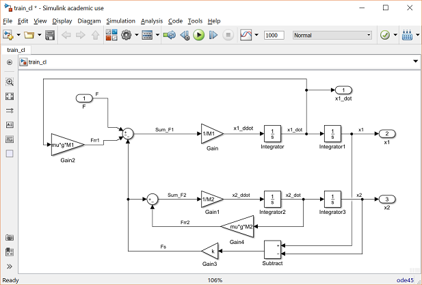
Next select all of the blocks in your model (Ctrl A) and select Create Subsystem from Selection after right-clicking on the model window. With a little rearranging and relabeling, your model will appear as shown below.

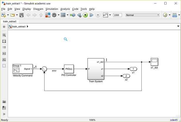
Now we can add a controller to our system. We will employ a PID controller which can be implemented using a PID Controller block from the Continuous library. Placing this block in series with the train subsystem, your model will appear as follows. In the following, we model the controller as generating the force "F" directly. This neglects the dynamics with which the train engine generates the torque applied to the wheels, and subsequently neglects the dynamics of how the force is generated at the wheel/track interface. This simplified approach is taken at this point since we only wish to introduce the basic functionality of Simulink for controller design and analysis.

Double-clicking on the PID Controller block, we will initially set the Integral (I) gain field equal to 0 and will leave the Proportional (P) and Derivative (D) gains as their defaults of 1 and 0, respectively. Next add a Sum block from the Math Operations library. Double-click on this block and modify the List of signs field to "|+-". Since we wish to control the velocity of the toy train engine, we will feed back the engine's velocity. This is accomplished by tapping a line off of the "x1_dot" signal and connecting it to the negative sign of the Sum block. The output of the Sum block will be the velocity error for the train engine and should be connected to the input of the PID Controller block. Connecting the blocks as described and adding labels, your model should appear as follows.

Next add a Signal Builder block from the Sources library to represent the velocity commanded to the train. Since we wish to design a controller to bring the train smoothly up to speed and smoothly to rest, we will test the system with a velocity command that steps up to 1 m/s followed by a step back down to 0 m/s (recall that our system is a toy train). To generate this type of command signal, double-click on the Signal Builder block. Then choose Change time range from the Axes menu at the top of the block's dialog window. Set the Max time field to "300" seconds. Next, set the step up to occur at 10 seconds and the step down to occur at 150 seconds. This is accomplished by clicking on the corresponding portions of the signal graph (left and right vertical lines) and either dragging the line to the desired position, or entering the desired time in the T field at the bottom of the window. When done, your signal should appear as follows.

Also add a Scope block from the Sinks library and use it to replace the Out1 block for the train's velocity. Relabeling the blocks, your model will appear as follows.

We are now ready to run the closed-loop simulation. If you wish to skip the above steps, you may download the completed model with control by right-clicking here and then selecting Save link as ....
Before running the model, we need to assign numerical values to each of the variables used in the model. For the train system, we will employ the following values.
 = 1 kg
 = 0.5 kg
 = 1 N/sec
 = 1 N
= 1 N = 0.02 sec/m
 = 9.8 m/s^2
Create a new m-file and enter the following commands.
M1 = 1;
M2 = 0.5;
k  = 1;
F  = 1;
mu = 0.02;
g  = 9.8;
Execute your m-file in the MATLAB command window to define these values. Simulink will recognize these MATLAB variables for use in the model. Next we need to set the time for which our simulation will run to match the time range of the command from the Signal Builder block. This is accomplished by selecting Model Configuration Parameters from the Simulation menu at the top of the model window and changing the Stop Time field to "300". Now, run the simulation and open the "x1_dot" scope to examine the velocity output. The result as shown below demonstrates that the closed-loop system is stable for this controller.
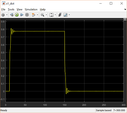
Since the performance achieved above is unsatisfactory because of steady-state error, we will show how to redesign our controller. We will first demonstrate how to extract a model from Simulink into MATLAB for analysis and design. Then we will demonstrate how to design the control from directly within Simulink.
The Simulink Control Design toolbox offers the functionality to extract a model from Simulink into the MATLAB workspace. This is especially useful for complicated, or nonlinear simulation models. This is also useful for generating discrete-time (sampled) models. For this example, let us extract a continous-time model of our train subsystem. First we need to identify the inputs and outputs of the model we wish to extract. The input to the train system is the force  . We can designate this fact by right-clicking on the signal representing "F" (output of the PID block) and choosing Linear Analysis Points > Open-loop Input from the resulting menu. Likewise, we can designate the output of the train system by right-clicking on the "x1_dot" signal and choosing Linear Analysis Points > Open-loop Output from the resulting menu. These inputs and outputs will now be indicated by small arrow symbols as shown in the following figure. Since we wish to extract a model of the train by itself, without control, we need to further delete the feedback signal, otherwise we will extract the closed-loop model from
  to
to  . Your model should now appear as follows.

We can now extract the model by opening the Linear Analysis Tool. This is accomplished by selecting Control Design > Linear Analysis from under the Analysis menu at the top of the model window. Following these steps will open the window shown below.

This tool generates an LTI object from a (possibly nonlinear) Simulink model and allows you to specify the point about which the linearization is performed. Since our Simulink model is already linear, our choice of operating point will have no effect and we can leave it as the default Model Initial Condition. In order to generate the linearized model, select the Step button in the above figure, which is indicated by a small green triangle. The Linear Analysis Tool window should now appear as shown below.

Inspecting the above, the step response of the linearized model was automatically generated. Comparing this step response to the one generated by the simulation of the open-loop train system in the Introduction: Simulink Modeling page, you can see that the responses are identical. This makes sense since the simulation model was already linear. Additionally, the linearization process generated the object linsys1 shown in the Linear Analysis Workspace above. This LTI object can be exported for use within MATLAB by simply dragging the object into the MATLAB Workspace portion of the Linear Analysis Tool window.
Having extracted this model, we can now employ all of the facilities that MATLAB offers for controller design. For example, let us employ the following commands to generate and analyze the closed-loop system reflecting the Simulink model created above.
         sys_cl = feedback(linsys1,1);
         p = pole(sys_cl)
         z = zero(sys_cl)
         p =

         -0.9237 + 0.0000i
         0.0000 + 0.0000i
         -0.2342 + 1.6574i
         -0.2342 - 1.6574i
         z =

         -0.0980 + 1.4108i
         -0.0980 - 1.4108i
         0.0000 + 0.0000i
Inspection of the above shows there is a pole-zero cancellation at the origin. Further, the remaining poles have negative real part and the two "slowest" poles are complex. This demonstrates that the closed-loop system in its current form is stable and the dominant poles are underdamped. This agrees with the result of our closed-loop simulation from above. We could then employ MATLAB to design a new controller in order to, for example, dampen out the oscillation in the response. In this case, we will rather demonstrate how to access some of MATLAB's functionality from directly within Simulink.
We can launch interactive tools to tune our controller from within Simulink. One manner in which this can be done is to double-click on the PID Controller in the model and select the Tune button to launch the PID Tuner tool. Rather than doing this, we will launch the more general Control System Designer tool by selecting Control Design > Control System Designer from under the Analysis menu located at the top of the model window. Following these steps will open the window shown below.

The first thing that needs to be done is to identify the controller block that is to be tuned. This is accomplished by first clicking on the Add Blocks button, and then selecting the PID Controller block from the resulting window as shown below. Next click the OK button. Note that controllers represented by other types of blocks (Transfer Function, State Space, etc.) can also be tuned.

Before we proceed to tune our controller, we must first identify the inputs and outputs of the closed-loop system we wish to analyze. This is done in a similar manner to how we extracted the linearized model into MATLAB. Specifically, right-click on the velocity command signal (output of the Signal Builder block) and choose Linear Analysis Points > Input Perturbation from the resulting menu to identify the input of our closed-loop system. Next, right-click on the train engine velocity signal ("x1_dot") and select Linear Analysis Points > Output Measurement from the menu to choose the output of our system. Your model should now appear as follows where the small arrow symbols identify the input and output of the model.
Now that we have identified the block to tune and our input and output signals, we can now commence with tuning the controller. Select the OK button in the Edit Architecture window. We should now be able to see the window shown below.

Clicking the Tuning Methods button, we will choose the design plots we wish to employ for designing our controller. In this example, we will employ a root locus design approach and hence will select the Root Locus Editor under Graphical Tuning as shown above. The root locus approach to design employs a plot that shows all possible closed-loop poles as a parameter (the loop gain) is varied from zero to infinity. Specifically, we make the following selection in the Select Response to Edit window and select Plot.

We then should obtain a root locus plot as shown below, which displays all possible closed-loop pole locations of the closed-loop train system under simple proportional control. Examining the plot, one can see that all values of loop gain will place the closed-loop poles in the left-half plane indicating a stable response.

If we decrease the loop gain sufficiently, we can move the closed-loop poles further into the left-half plane and we can change the performance of our system. This can be accomplished graphically by "grabbing" the pink boxes marking the closed-loop pole locations and dragging them toward the open-loop pole locations (marked by x's). We can examine the corresponding closed-loop step response by clicking on New Plot under the CONTROL SYSTEM tab and selecting New Step. When the following window appears, we then select New Input-Output Transfer Response from the Select Response to Plot dropdown menu as shown.

Then we specify the input and output signals within the New Step to plot window as shown below.

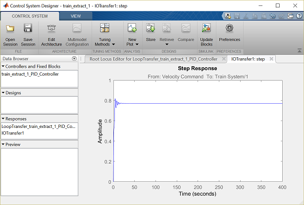
Then click the Plot button. From the resulting closed-loop step response we can see that the response is stable, but with some steady-state error.
Recall that adding integral control is one way to reduce the steady-state error of a closed-loop system. In this case, adding an integrator via the controller will make the system type 1, where type 1 systems can track step references with zero steady-state error. Recall the following form of a PI controller.
(1)
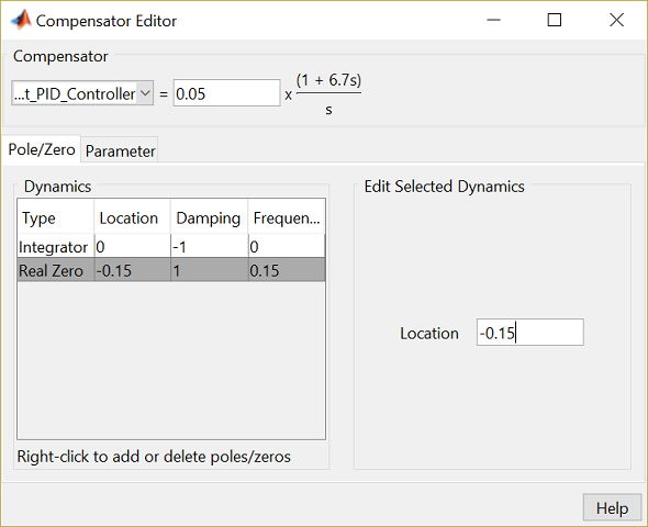
Inspection of this equation demonstrates that a PI controller will add an integrator and a zero to our open-loop system. The integrator can be added to the system by right-clicking in the field of the root locus plot and selecting Add Pole/Zero > Integrator from the resulting menu. Similarly, the zero can be added by right-clicking on the root locus plot and selecting Add Pole/Zero > Real Zero from the resulting menu. Then click on the real axis where you wish to place the zero. You can move the zero by clicking on it and dragging it to a new location. The compensator can also be edited by directly typing in pole and zero locations. This can be achieved by right-clicking on the root locus plot and choosing Edit Compensator from the resulting menu. The window that opens is shown below. We will place an integrator, a real zero at -0.15, and will choose a loop gain equal to 0.05.
The resulting closed-loop step response plot is shown below demonstrating that the train engine is brought to rest smoothly and with zero steady-state error for a constant speed command.
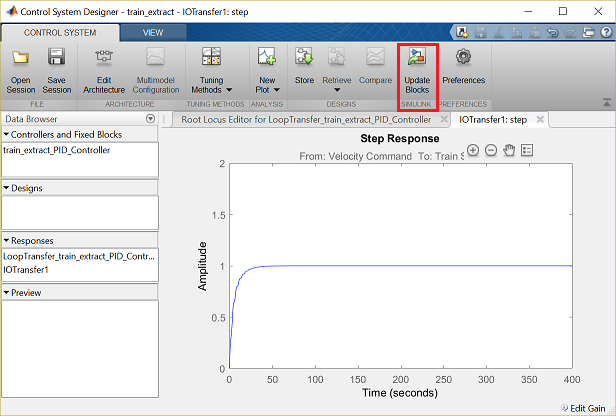
The control gains that have been chosen can then be applied to the Simulink model by clicking the Update Blocks button within the CONTROL SYSTEM tab as shown above. The simulation can then be run with this newly tuned controller. Clicking on the Scope block for the train engine's velocity will produce a plot like the one shown below.
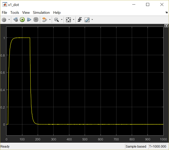
Overall, this response seems to meet our goals of bringing the train up to speed and back to rest smoothly, while maintaining minimal steady-state error. This response matches the result generated with the Control System Designer above because that analysis and the Simulink model used the exact same linear model.